How to solve PDE efficiently, and finding functions that fail the second partial derivative test

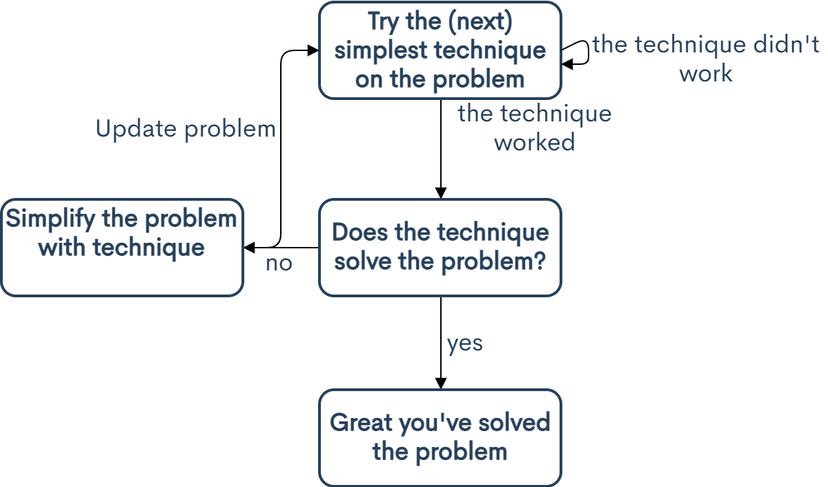
     Hello. The question I want to answers with this post is, without a good intuition of when to use techniques you've learnt, how do you solve a problem efficiently? To do this I propose a framework we'll call sequential solving, which you can see in the flowchart below. You start with the simplest technique you think will work and check if it simplifies the problem. If the check fails keep repeating those steps, each time using the next simplest technique until you find a technique that simplifies the problem. Then keep repeating that whole process with your simplified problem until you reach a solution.

    The main benefit of this framework is that you use the simplest techniques that works, meaning you don't have spend more time than necessaire solving the problem. Obviously if you have a good intuition for which techniques to use, use your intuition. In most topics you usually have a good intuition because there's only one maybe two good ways to solve a given problem, but in differential equations there can be a half dozen ways to solve a single problem. As such the example of using this framework will be a differential equation. For those of you who haven't studied the subject before you go here's my pitch for the subject. Most real world systems can only be modeled by differential equations ie gravity, electromagnetism. And for those of you that know the second partial derivative test, below are functions which fail the test at very point where g is an arbitrary differentiable function. Which of course is derived by using differential equations. If you have the time I would highly recommend learning the subject. Okay bye.

    Before we go to the example here’s what the order of techniques I use looks like when sequentially solving PDE. 

Trivial solutions

Separable equations

Separation of variables

Laplace or fourier transform

Method of characteristics

Similarity of solutions

   Additionally within each technique try simplify algebraically and by grouping derivative terms ie below.

    Now let's dig in to sequentially solving in practice. Were going to find functions which fail the second partial derivative test, from now on spdt, at every point(not just critical points). For a refresher, the spdt categorizes critical points (x₀,y₀) of a function f(x,y) by the value of h. The important thing for this example is that when h=0 the spdt fails.

    Plugin in h=0, let's call this equation *.

  *

    Now the first step on our list, trivial solutions. I notice two ways to construct trivial solutions here so let's try them both. For the first trivial solution let’s set both sides  of * equal to zero.

    Lets think about when these equations are satisfied. Notice that we’re taking the derivative with respect to both variables in each derivative expression. So if we don’t have any dependence on one variable both of the derivative expression will go to zero. Then our solutions is a function dependent on only one variable. To note from here forward g is arbitrary differentiable single variable function.

    Now let's look at the other trivial solution; setting the mixed partial derivate equal to the xx and yy derivatives.

    Now what methods could we use to solve this simplified problem? For clarity and time we'll skip trying separable equations, separation of variables, and transform techniques as even though they look like they'll work they give us non-general answers. Moving on to the method of characteristics let’s find the characteristic curves using the parameter t. 

    So we get are characteristic curve and then our solution follows.

    

    A solution of this generality would suffice for most practical applications, but for practice let's find a more general solution. * definitely isn't separable, I don't think separation of variables would give us a general answers, it's not linear so we can’t use laplace or fourier transforms, it's not first order so we can't use method of characteristics, but ah similarity of solutions would work.  For similarity of solutions let’s first find transformations under which * doesn't change.

    To make both side equal we have to cancel out the ɛ term. So 2a+2b-2c=0 which doesn’t give us any information about the relative value between a/b and c/b. So let’s reuse the variables a and b to get a form of function which reduces to an ODE when plugged into *. We'll call this function •.

  •

    Plugin • into * after some harry algebra, and dropping the argument of h from g(h) we get.

OH that's really nice. In your head plug in a=1 ,b=-1. It just all goes to zero nicely. Plugging those value of a,b into • we get the solution to the left. The solution to the right follows by the same argument with x and y swapped in •. Also to note, we go the same result as the first trivial solution for a,b=0. 

 

    This is a very satisfying result, does it give us some deep insight into the nature of critical points? No, I assume this has more to do with spdt itself then anything intrinsic to critical points. However, it was still a good example of using sequential solving to efficiently find solution to a problem. For a challenge try solving the problem below using sequential solving, remember to look at the order of techniques before diving in. 

The practice problem above is from https://www.math.ucla.edu/~yanovsky/handbooks/PDEs.pdf a great resource with tons of other differential equation problems. Solution on page 86.